Project Log
Ideas and uncategorized artifacts
2025-01-13 — Counting codepoints in UTF-8
✋ This blog describes an "aha!" moment I had reading a UTF-8 codepoint counting implementation. It describes how that code works, but this isn't a post primarly about low-level UTF-8 optimizations. There may be more efficient algorithms, but I thought this one was interesting.
While refactoring some string processing code in the Mojo🔥 standard library, I came across an interesting piece of logic used for counting the number of codepoints that are stored in a UTF-8 encoded string. But, before I describe what I found interesting about the algorithm, first a brief medium-length refresher on the byte-level structure of UTF-8 encoded text.
In the UTF-8 encoding, all characters are assigned a codepoint, whose integer value is encoded using between 1-4 bytes. (The fact that different codepoints can encode to byte sequences of different lengths makes UTF-8 what’s known as a "variable width" encoding.)
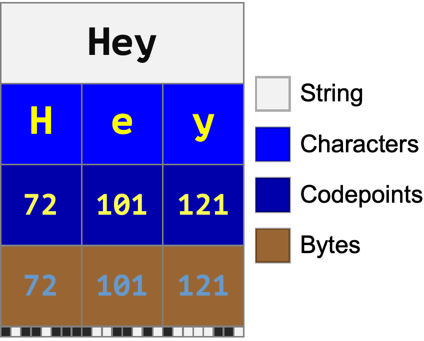
For text using the Latin script, typically most or even all characters are encoded using a single byte:
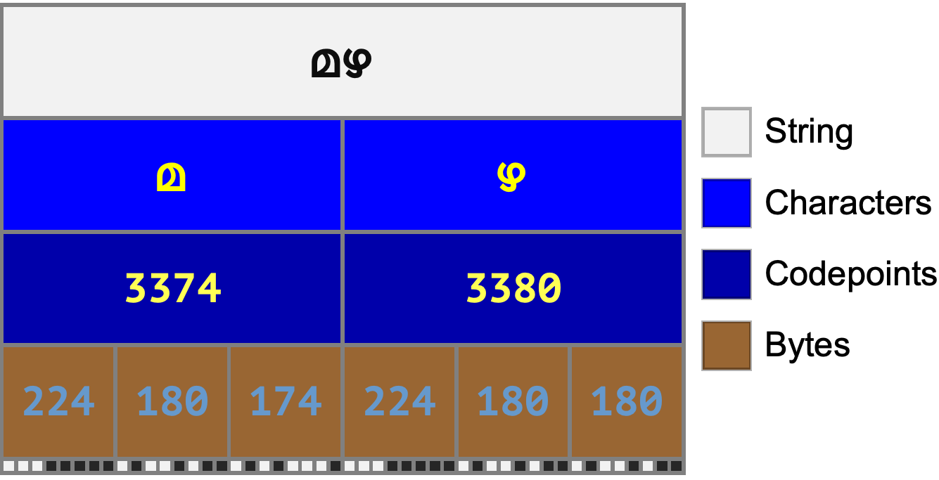
On the other hand, characters in non-Latin-alphabet languages may encode to longer byte sequences:
An important outcome of the choice to make UTF-8 a variable-width encoding is that you can mix and match characters from different scripts—something we take for granted today (but which wasn’t easily possible in the days of 8-bit character encodings):

But, because there’s no way to know ahead of time how many bytes are in each character, UTF-8 has to store the length of each and every codepoint inline in the binary data. This also means that counting the number of codepoints requires a linear scan of the entire string contents. To understand the implementation of codepoint counting mentioned at the beginning of this post, let’s take a closer look at exactly how the bits and byte values of UTF-8 text are stored.
Every byte in UTF-8 encoded text can be categorized into one of 5 types. Each byte type has a distinctive bit pattern in its leading bits:

From the table above we can see that, in UTF-8, all single-byte (ASCII) characters start with the bit 0. We can check this is true by looking at the bit pattern of the ASCII character ‘R’:
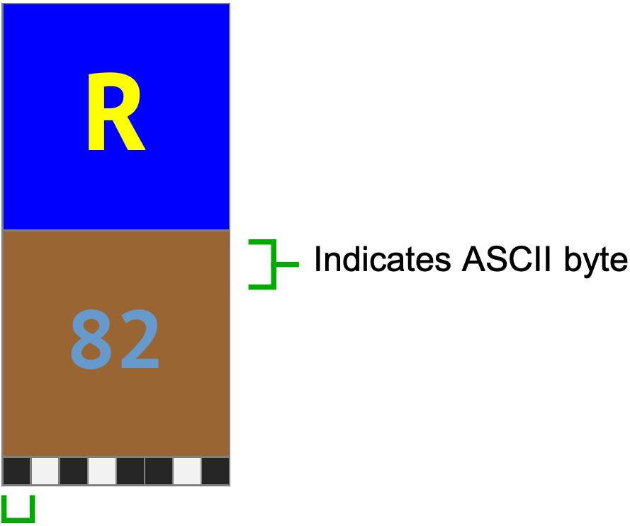
However, multi-byte codepoint sequences have a more complicated structure. In a multi-byte sequence, the first byte encodes the length of the sequence in the number of leading 1 bits, and the following bytes are continuation bytes.
Let’s check our understanding by looking at a multi-byte character that has 3 bytes. Based on the table above, we’d expect the first byte to match the bit pattern 1110xxxx, and that’s exactly what we see:
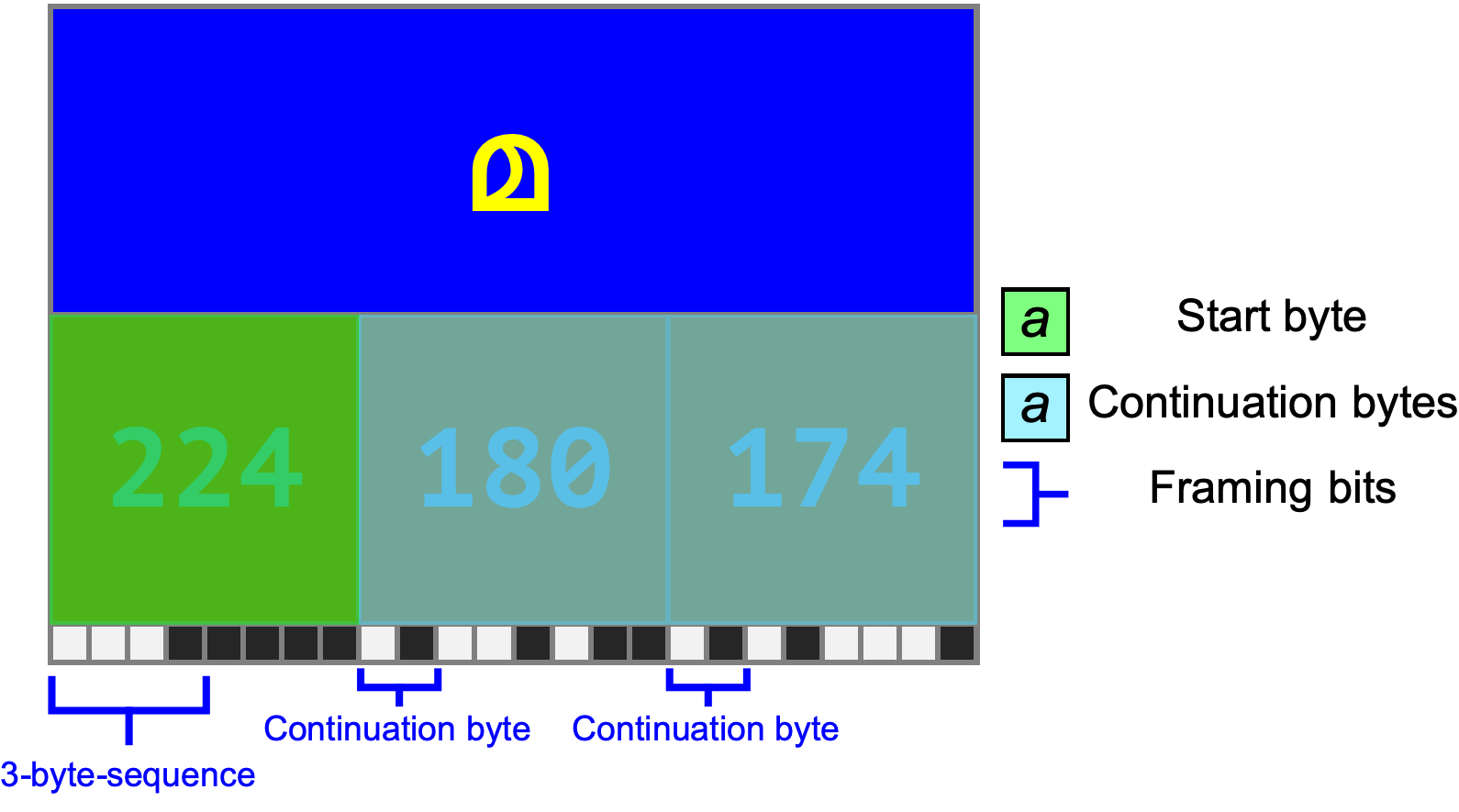
We also see that, as expected, the continuation bytes match the bit pattern 10xxxxxx.
So, now that we understand how to distinguish the different byte types in a UTF-8 codepoint sequence, how can we count the overall number of codepoints?
One thing we might try is counting every “leading” byte — since every code point has one first byte that encodes it’s length, we just need to identify and count all those “first” bytes, and ignore the continuation bytes. As a refresher, here’s the table again showing the byte type bit patterns:
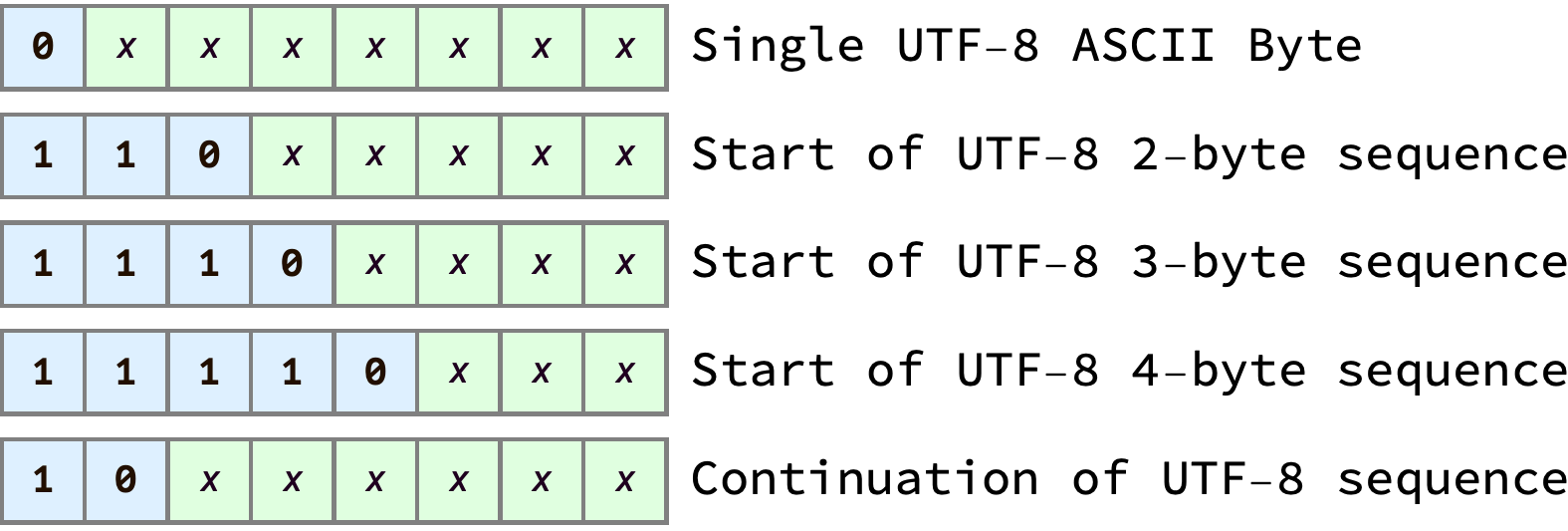
Counting the leading bytes would be the same thing as counting any bytes that match the four “first” byte patterns above, i.e. counting any bytes that start with either 0x, 110x, 1110x, or 11110x. Writing efficient low-level bit twiddling code to check if a byte matches any of those patterns is not trivial.
However, if we think about this problem another way, an elegant and obvious-in-hindsight solution reveals itself (a solution perhaps so obvious future readers might ask if it really warranted writing a blog post about it; perhaps not, but it was a pleasing “aha!” moment for me): count the continuation bytes instead.
If we again study the chart above, we can see that identifying continuation bytes can be very efficient: Just check if the number of leading 1’s in a given byte is equal to 1. There are efficient instructions on all modern processors to count the number of leading zeros, so a bitwise NOT (^) followed by a "ctlz" instruction will tell you the leading 1 count.
Once the number of continuation bytes is counted, all that’s left to calculate the number of codepoints is to subtract that continuation byte count from the total byte count of the string.
For a “physical” intuition of why this is correct, lets have another look a piece of text, containing a mix of 1, 2, 3, and 4 byte codepoints. If you know the total byte count and can quickly count the continuation bytes then you can subtract to get the number of start bytes: 13 - 8 = 5. And as we know the number of start bytes is equal to the number of codepoints, and we’re done.

Credits: Thank you to my friends Jacob and Manu for proofreading the Malayalam text in this post🙂
2025-01-09 — Unicode scalar values
While working on adding a Char type to the Mojo🔥 standard library, I realized that, although I’ve read the definition of "Unicode scalar value" many times, I didn’t have a great intuition for what it actually “looked like” in the context of the full range of Unicode code points.
Unicode has a theoretical maximum capacity of ~1.1 million codepoints (up to the maximum codepoint value of 0x10FFFF). “Scalar values” are the codepoints in the subset of that range that excludes the "surrogate" codepoints, which are reserved codepoints used by the UTF-16 encoding for backwards compatibility. So, excluding the surrogate code points, what codepoints are left that are called “scalar values”?
Looking at the full range of ~1.1 million codepoints, the surrogate codepoints look like a dot, a very small part of the full range:

If we zoom in on the portion of the range containing the surrogate codepoints, we can see that all surrogate codepoints fall in the range 0xD800 ≤ surrogate ≤ 0xDFFF, and are further split into the "high" surrogates and "low" surrogates:

This gives a nice visual intuition for what it means to validate that an integer is a valid Unicode scalar value: less that 0x10FFFF, and not in the range 0xD800 – 0xDFFF.
2024-12-01 — Machine code diagramming experiments
Today I’ve finally gotten back to picking up work on machine code diagramming (which I started in August, but then spent several months yak-shaving on Diagrams core functionality and new authoring utilities).
This is very rough, but the doodling below shows the outline of what is possible:
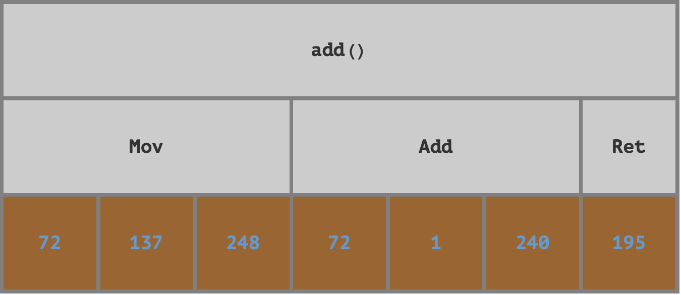
TreeStackDiagram.In my opinion, this is a great example of how notebooks can leverage the bringing-together of many heavy-weight component libraries to achieve a result that is pedagogically quite potent.
Consider what’s being done: We’re writing real, running code that demonstrates how several low-level computing concepts directly relate to each other in a computational—concrete—way: IR is a way of writing code; libraries like LLVM can compile IR into an executable format; other libraries (merely) know how to parse that format and extract information from it; and we can visualize the layers of abstraction present in machine code (raw bytes encode instructions; functions are made of blocks of instructions; executable files are ~groups of functions).
define i64 @add(i64 %x, i64 %y) {
    %1 = add nsw nuw i64 %x, %y
    ret i64 %1
}

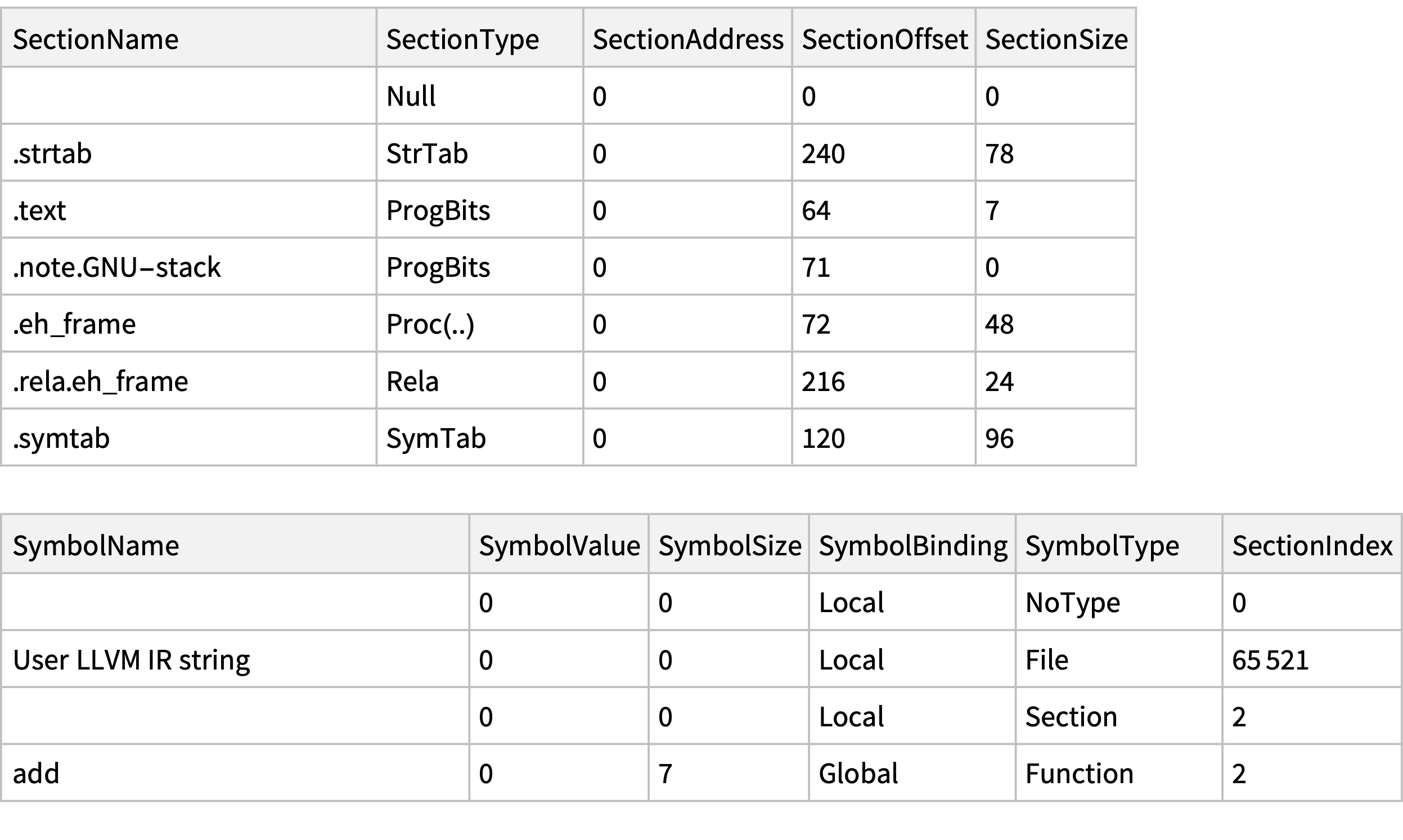
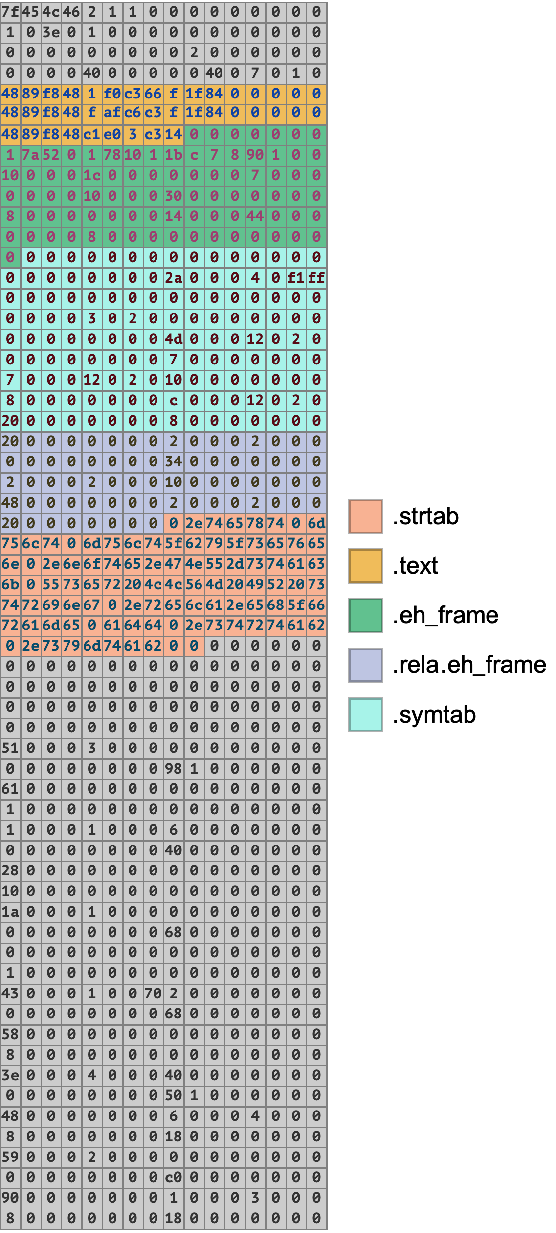
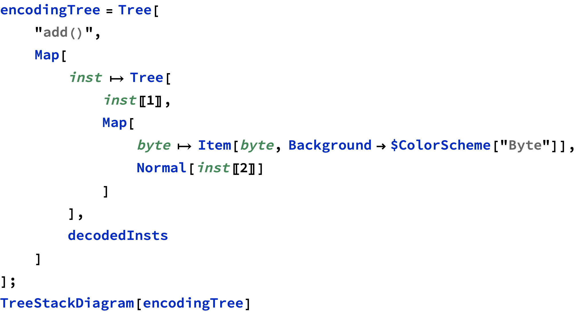
add() function, we first need to calculate its position in the overall object file byte buffer: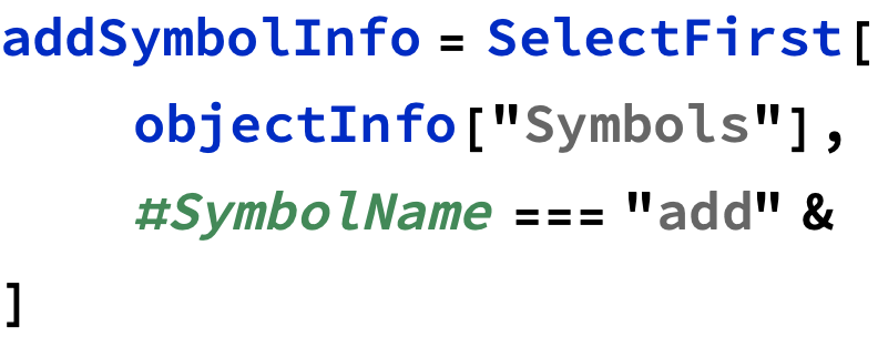
add() (+1 to account for 0- vs 1-indexing; -1 because Span is inclusive but the size forms a half-open range):

2024-10-07 — DiagramLegend utility
I whipped together a little utility to help with adding legends to diagrams:
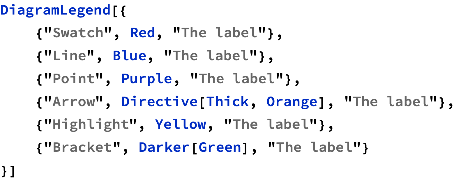
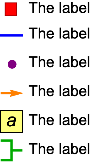
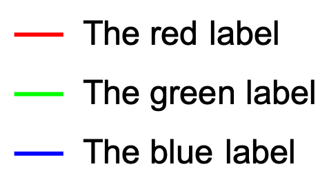
This generalizes over (and extends) the existing built-in legending forms in Wolfram, which are specialized to the visual type of legend: SwatchLegend[..], LineLegend[..], PointLegend[..], e.g.:

2024-10-03 — Notes on geometry visualization in Wolfram
While working on the problem of arrow placement in Diagrams (see horrible arrow placement in previous log entry), I got sidetracked with thinking about angle computations, and built a couple of utility functions.
It was a bit of a rabbit hole, because after getting the arrow placement math more or less working, I wanted to build a widget to explain that math (the subject of the previous log entry). While doing that, I realized that the calculations needed to visualize the problem were slightly different from the calculations needed to solve the problem — to do the visualization, I couldn’t just reuse the formulas from the computation function, I needed new functionality!
This entry describes part of that new functionality, a utility I wrote called CircularArcThroughAngles. (A subsequent post will describe the even lower level function I wrote, called AngleDifferences).
Consider the problem of finding the “difference” between two angles (visualized as radial lines at that angle):
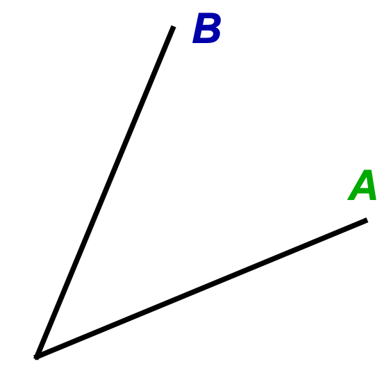
What differences can we think of between A and B?
Additionally, do we need to know the direction we need to rotate, or do we only want the absolute magnitude of the difference?
Another question we could ask is: what do we need to know to visualize the arc formed by the two angles shown?
As far as I can tell, there isn’t (yet) a single function in Wolfram that can be used to answer all of the above questions.
First problem: There is no dedicated function in Wolfram to get the difference between two given angles. (A simple difference is just B - A, but that doesn’t do the adjustments needed for specific use cases).
For the visualization problem, the third argument of Circle looks promising:

Let’s try it:
The first example below is okay, but the second example isn’t what we want, because its showing a “full exterior” angle, when we want to visualize the “interior” angle, because the “interior” angle captures better the intuition of “how far is the second angle from matching the first angle”.
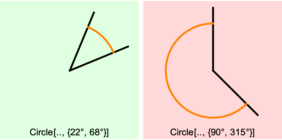
An interesting thing here is that the “interior” angle needs to be a signed value for us to visualize the intuition that its the absolute magnitude of the difference between the two angles that matters.
Correspondingly, we might show the absolute angle as text, and use the absolute angle as part of the arrow placement computation, while still using the signed angle as part of the visualization logic.
That’s an interesting case where the value needed to visualize a phenomenon is just fundamentally not the same as the value needed to do related computation.
So, Circle didn’t work for us. What about PlanarAngle?
PlanarAngle looks promising, because it provides a “spec” option we can use to choose which output we want:

Alas, PlanarAngle works only on points, and it has no specification to return signed angles, making it not the right choice for certain visualization tasks, where knowing which direction the angle needs to go away from a particular point is needed to actually draw that arc on the screen.
To fix this, I wrote my own utility function, CircularArcThroughAngles:
CircularArcThroughAngles[a1, a2, center, radius, spec]
CircularArcThroughAngles always returns a Circle, but allows the user to specify the kind of arc that should be returned:
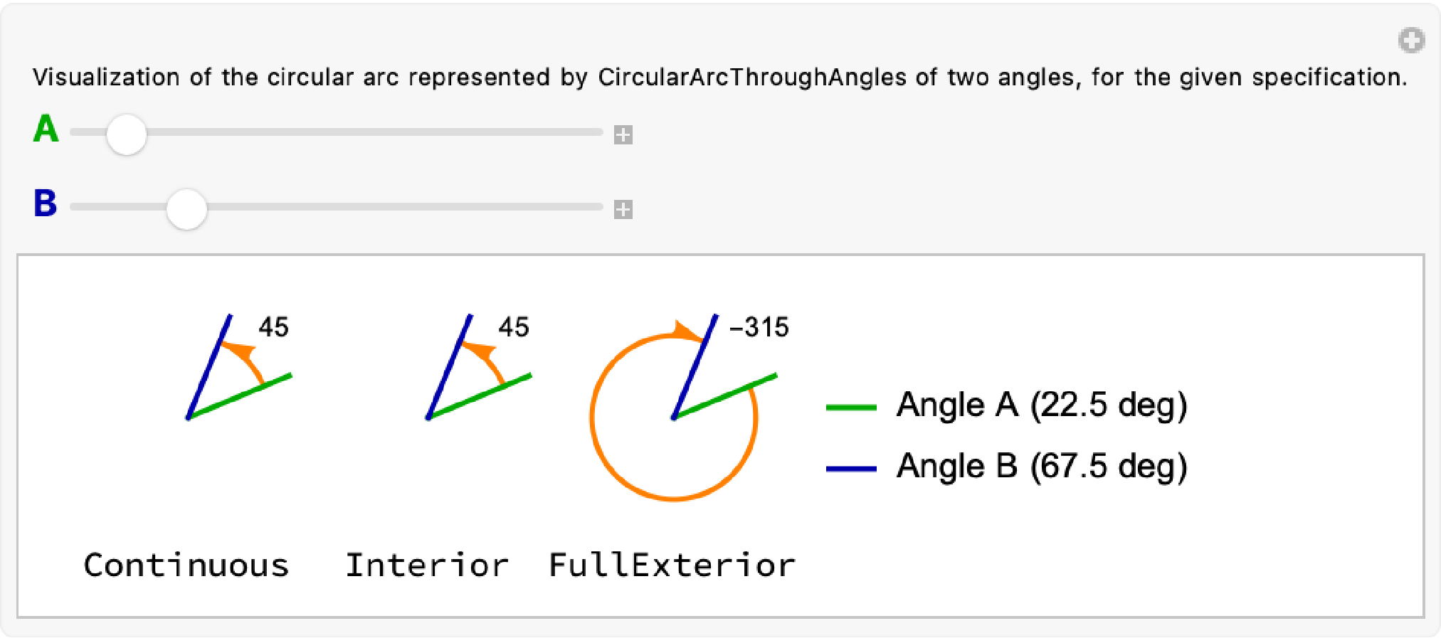
The magnitude of each angle difference is shown in text, and includes the sign (direction) of the change in angle needed to go from Angle A to Angle B, in the direction specified by the spec values shown labeling each figure (“Continuous”, “Interior”, “FullExterior”).
To better illustrate the difference between “Continuous” and “Interior”, consider an alternate case where A is at 0 degrees, but B is at 215 degrees.
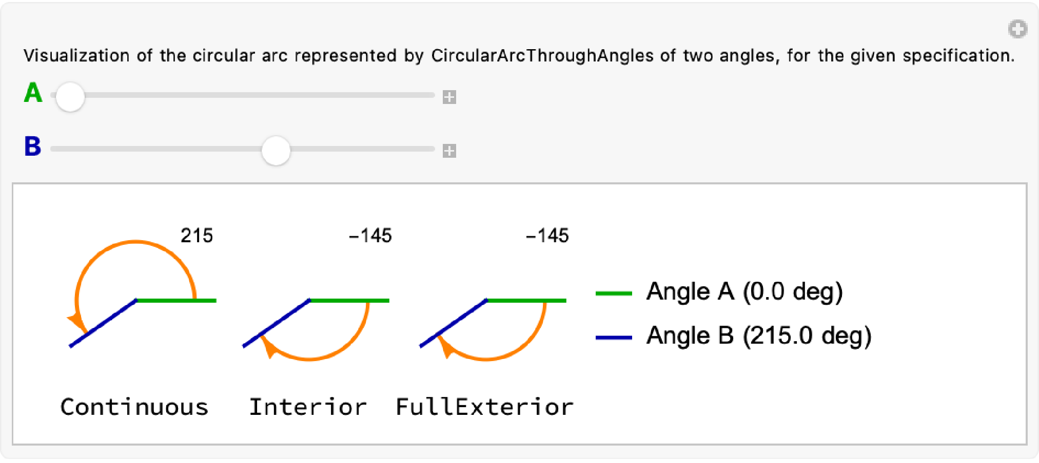
In the example above, the “Continuous” difference between A and B is 215 degrees: A would have to rotate another 215 degrees to be equal to B.
But the “Interior” arc between A and B is no longer the same as “Continuous”. Instead, the “Interior” arc is always an arc starting at A and rotating towards B in whichever direction is shortest. In this case, a -145 degree, clockwise turn from A towards B is “closer” than the alternative counterclockwise that “Continuous” represents.
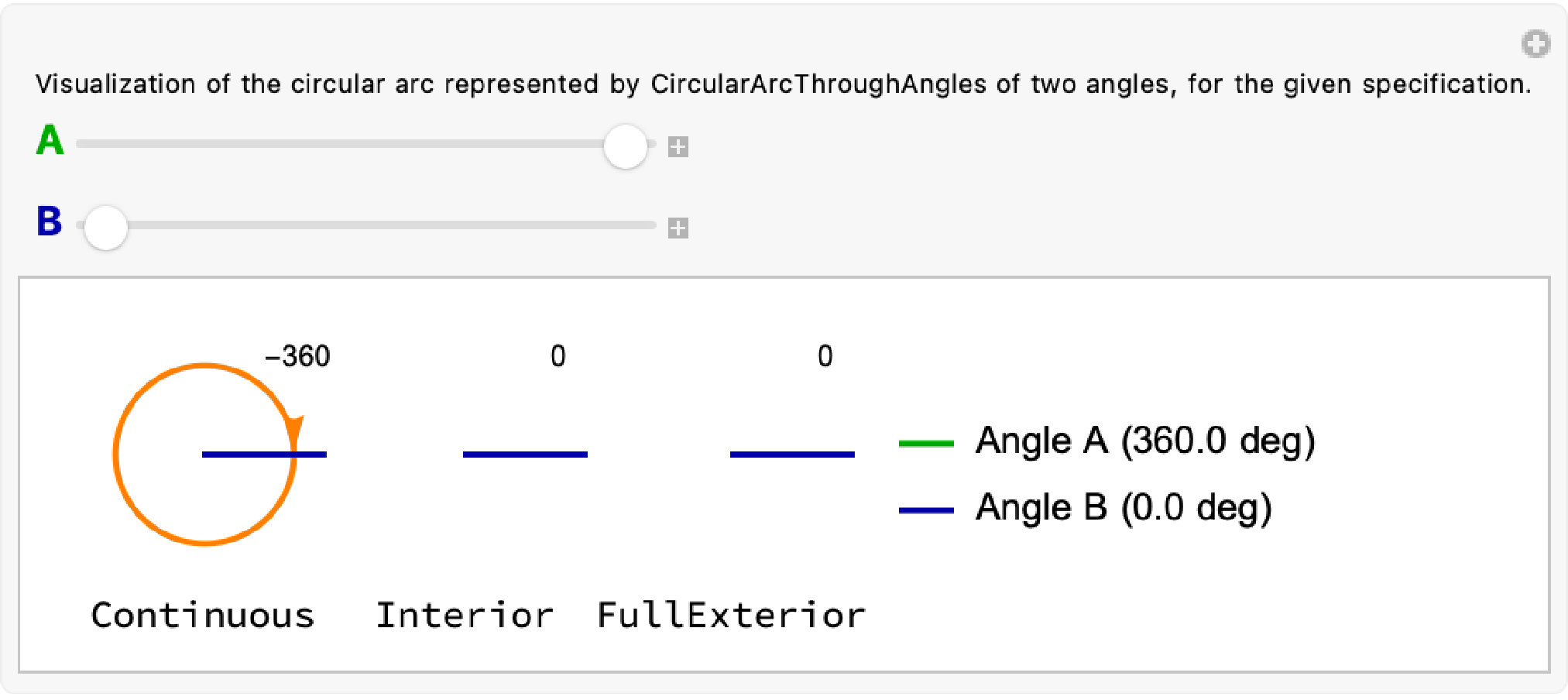
Consider as well an extreme case:
2024-09-24 — Adding margins
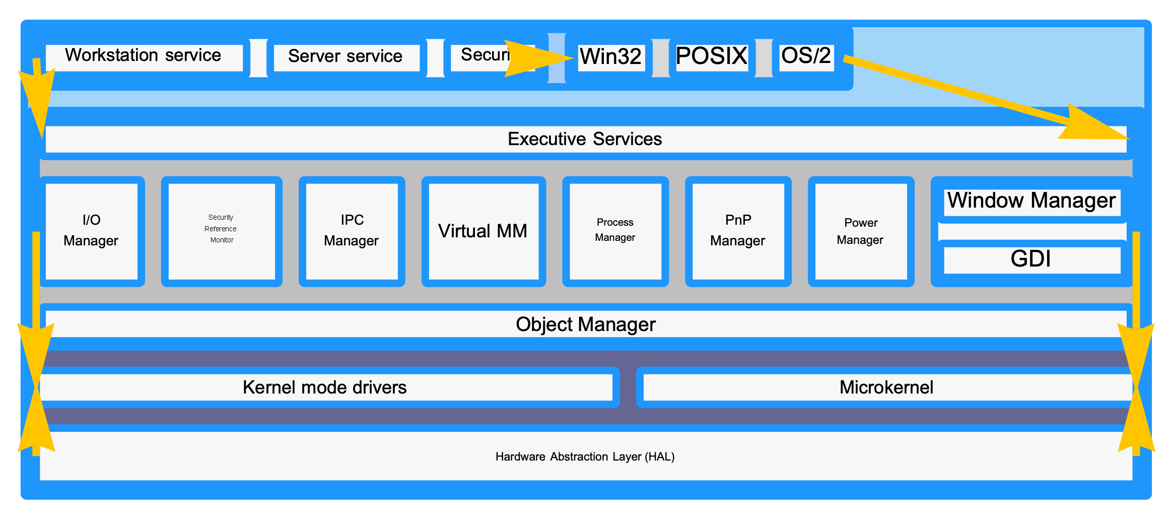
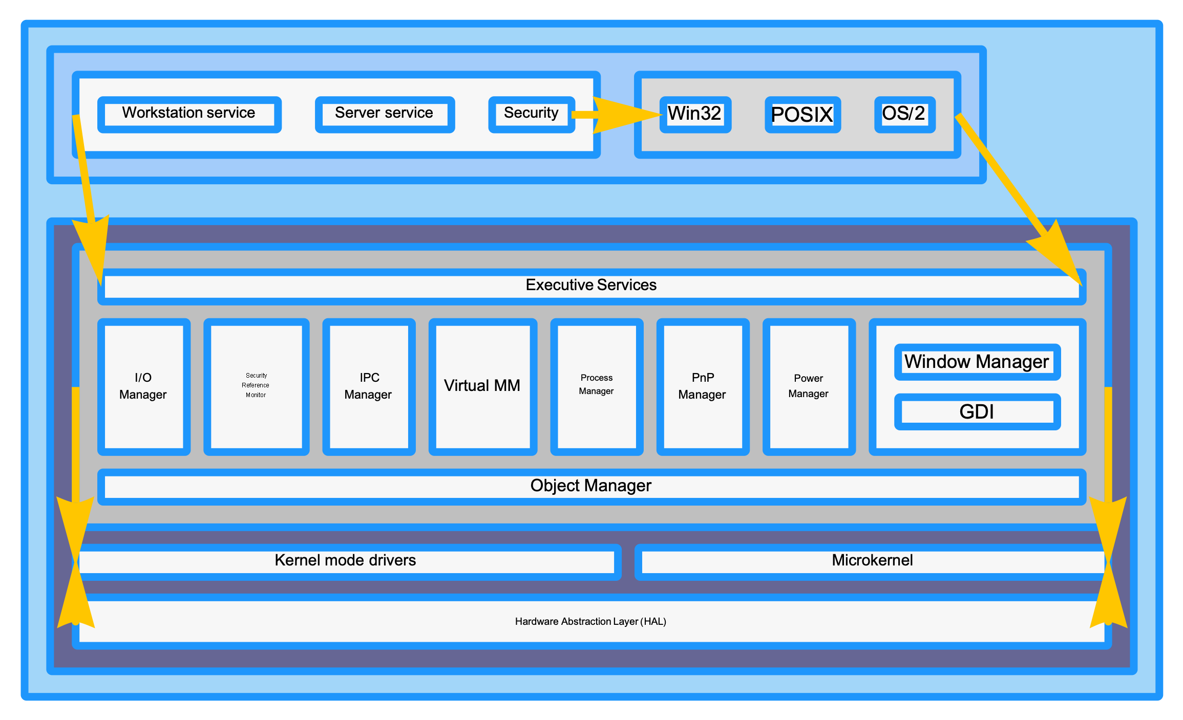
Last night I was playing around with implementing support for “margin” on boxes in BlockDiagram, and made a nice visual improvement to the Block-10-WikipediaBlockDiagramWindows test case. This is the first version of that diagram where its almost plausible that its a “real” diagram, not something half-finished.
(The next major improvement is to fix the SizedText algorithm so that multi-line labels aren’t tiny. And fix the placed arrows layout algorithm to account for arrow angle. And maybe add margin collapsing to avoid double counting margin in Row and Column; though that’s a more marginal improvement 😉.)
Old:
New
2024-09-15 — Hierarchical Layout
Up to this point, Diagrams only supported a single top-level DiagramLayout option for controlling the layout of diagram elements. Now, diagrams supports a ContentLayout[content, layout] symbolic wrapper, for specifying the layout algorithm that should be used to lay out the specified content:
As an example of what this enables, consider the following diagram specification:
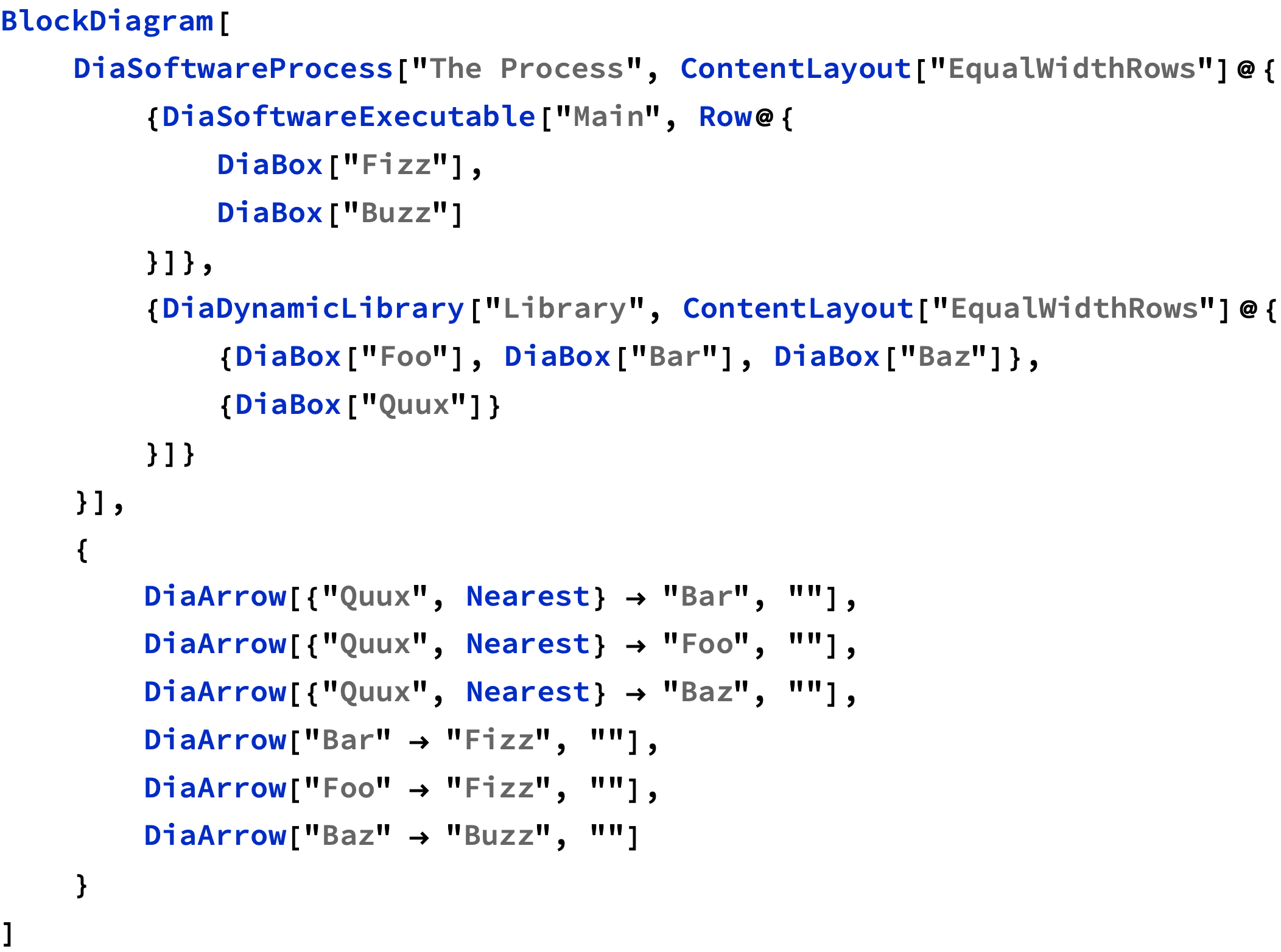
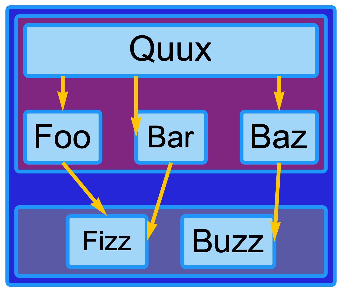
This diagram has several levels of hierarchy:
Row[{...}] specification, which the “Quux”, “Foo”, “Bar”, and “Baz” elements are themselves laid out using another instance of the “EqualWidthRows” algorithm, forcing the “Quux” box to be much wider than it otherwise would have been.I’m excited about this change because it will allow a user to strike a balance between using automatic layout in the cases where it can work well, with the precision afforded by specifying layout manually. There is much more to build, but this is a nice first step.
2024-08-28 — Notes on ASCII tree drawing
I was pleased to find out that getting a basic ASCII text version of FileSystemTreeDiagram working only took a couple of hours this evening:
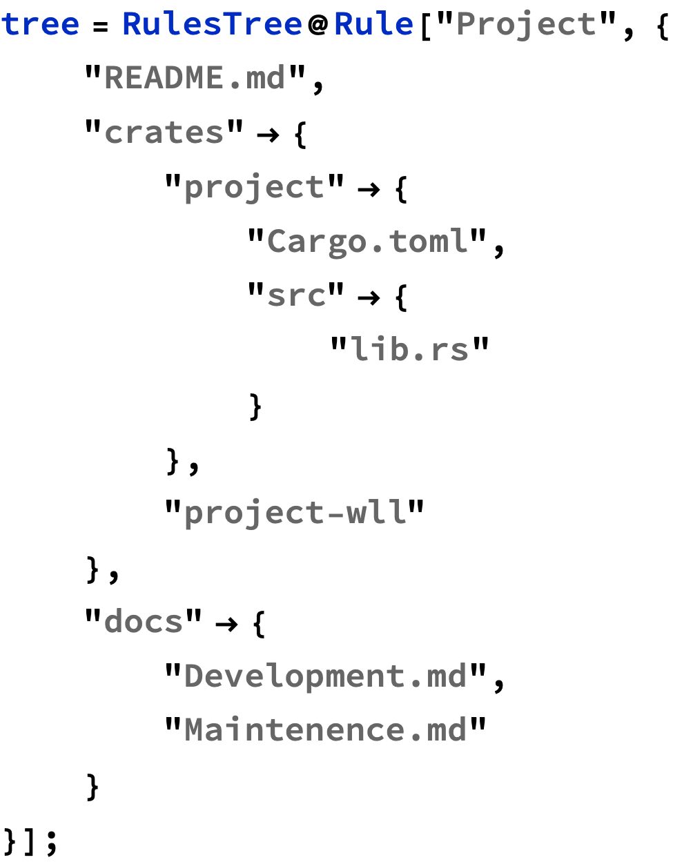

The tricky part was figuring out the right recursive-ish algorithm (and data structure along with it) to know the state needed to render each line.
Initially I tried a purely recursive algorithm, where the complete text of each subtree got created and then “indented” to start rendering at a higher level in the tree. This was somewhat error prone (not to mention inefficient) because it required fiddly text processing to split on newlines (and later rejoin) many times over.
What I ended up with is a stateful algorithm that maintains a single string that is the output text, and then executes a recursive top-down traversal of the nodes. Each recursion is a call to a `visit` closure function that can write directly to the output string buffer.
The only data structure needed is a “stack” of booleans, where:
This approach generates a data structure that looks like this. The column of text on the right is the state of the boolean value “stack” at the time the node on that line is written out.
Project                       {}
|-- README.md                 {False}
|-- crates                    {False}
|   |-- project               {False, False}
|   |   |-- Cargo.toml        {False, False, False}
|   |   \-- src               {False, False, True}
|   |       \-- lib.rs        {False, False, True, True}
|   \-- project-wll           {False, True}
\-- docs                      {True}
    |-- Development.md        {True, False}
    \-- Maintenence.md        {True, True}
This boolean “stack” ends up being one of two pieces of data needed to draw the lines of the tree.
The key insight is that the lines can actually be thought of as discrete “cells”, each 4-characters wide, and arranged in rows and columns.
Each row can be processed independently. But within a row, the “inner” (left-most) columns and the single “outer” (right-most) column need to draw slightly different characters. The table below shows which 4-character cell “value” is written based on the state in each {row, column} position.
| Inner Column | Outer Column | |
|---|---|---|
| Non-Last Sibling (False) | "| " | "|-- " |
| Last Sibling (True) | " " | "\-- " |
Where a “column” is one of the 4-character wide spans highlighted in the graphic below. Also highlighted is how the boolean values as well as the “inner” vs “outer” position of the column maps onto the 4-character spans chosen from the table above:
Project                       {}
|-- README.md                 {False}
|-- crates                    {False}
|   |-- project               {False, False}
|   |   |-- Cargo.toml        {False, False, False}
|   |   \-- src               {False, False, True}
|   |       \-- lib.rs        {False, False, True, True}
|   \-- project-wll           {False, True}
\-- docs                      {True}
    |-- Development.md        {True, False}
    \-- Maintenence.md        {True, True}
2024-08-24 — Saturday
I’ve got the basics of compiling LLVM IR from a notebook into X86-64 assembly working:
define i64 @add(i64 %x, i64 %y) {
    %1 = add i64 %x, %y
    ret i64 %1
}

2024-08-21 — Wednesday
We just got back from a trip to Utah, and rode for ~40 hours on Amtrak.
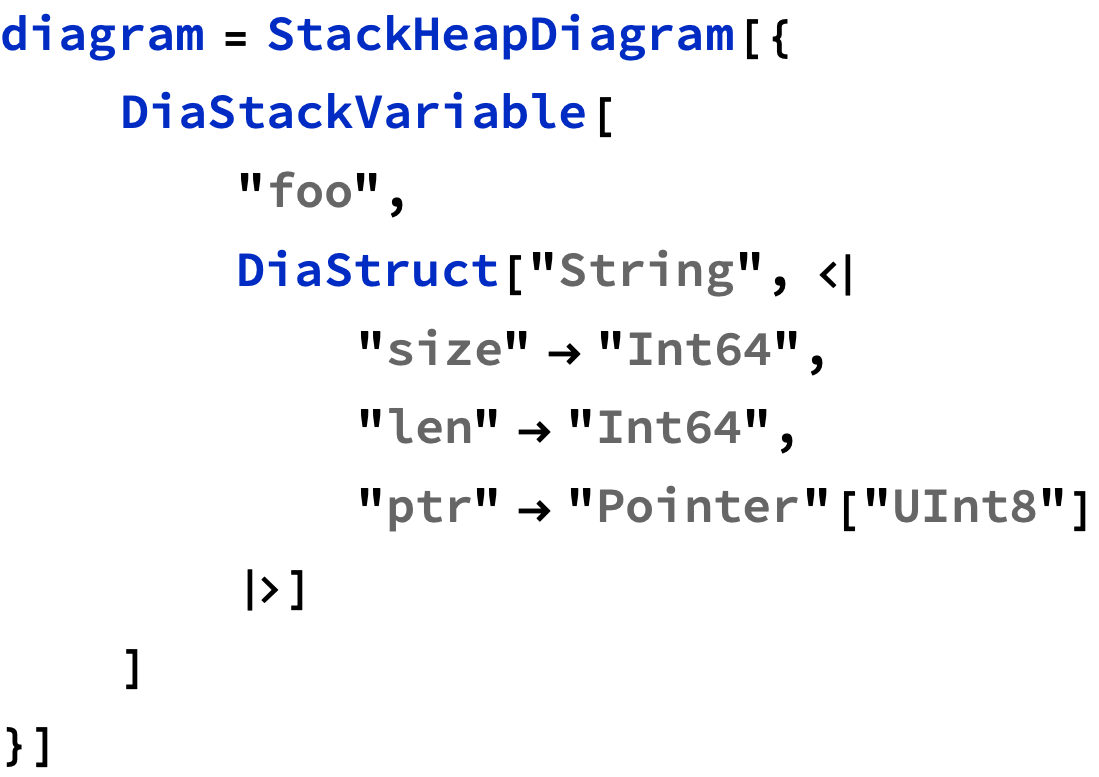
The time on the train gave me a chance to put the finishing touches on a new DiagramAnnotate[..] prototype:


2024-08-10 — Saturday
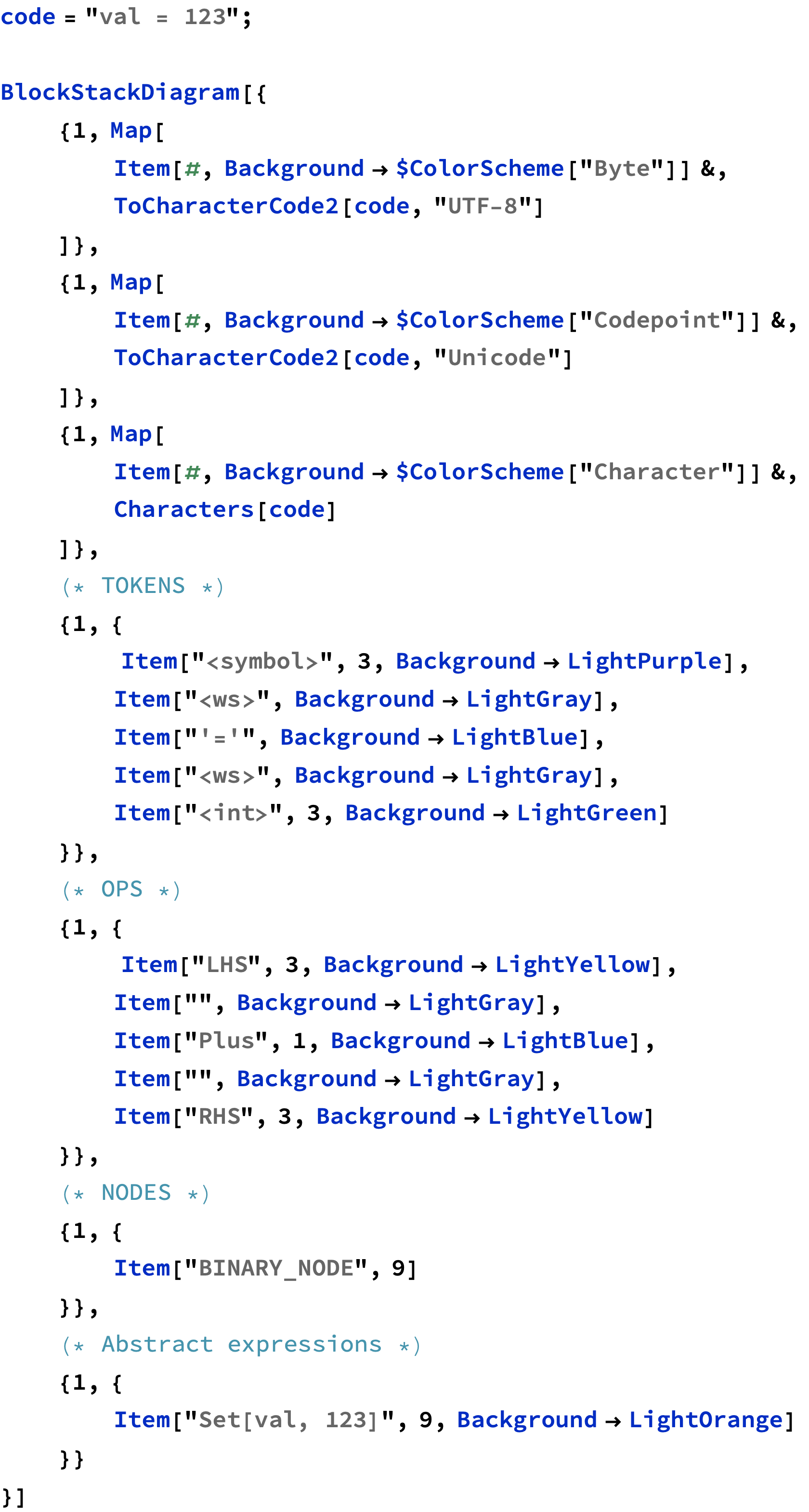
Today I’ve been continuing work on “program diagrams” in Diagrams (/project/Diagrams), and finally crystalized an example of the idea I’ve had for a while to build on top of StringEncodingDiagram with something like “ParseDiagram”.
This is still pretty verbose because it hasn’t actually been factored out into a function, but I think the result is on the right track:
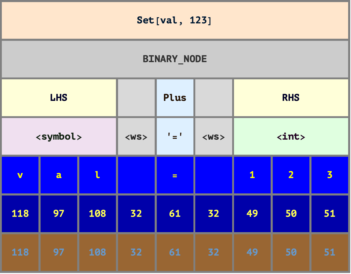
Future work will be to factor this out into the aforementioned ParseDiagram function, and support nice convenience integrations like ParseDiagram[CodeParse[“...”]].
I.e, it should be possible to pass the following result directly to ParseDiagram:

On a related note, I was thinking an animation to show how lexing / tokenization generally happens “linearly”, but parsing happens in a tree-wise fashion could be interesting. Imagine for example that the layers of the earlier diagram got “built up” incrementally from the token layer up and from left to right.
The intent would be to give intuition to why parsing is typically much more complicated than tokenization. Much has been written about parsing strategies: Shunting yard, Pratt, context-free, LL(1), LL(N), recursive descent, etc. are all concepts that might come up researching parsing. But the relatively lesser complexity of tokenization doesn’t invite the same multiplication of jargon that parsing does.